Finding a good reward function for optimal policy in reinforcement learning is often challenging, and Inverse Reinforcement Learning(IRL) handles this limitation very well. In IRL, we try to find the agent’s objective, optimal reward function based on behaviour or demonstration from the past and bootstrap the learning process.

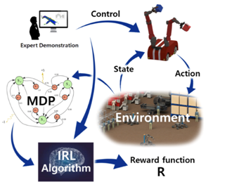
In this article, we are going to discuss one such algorithm-based Inverse Reinforcement Learning. The proposed MBIRL algorithm learns loss functions and rewards via gradient-based bi-level optimization.  This framework builds upon approaches from visual model-predictive control and IRL. This new MBIRL algorithm is a collaborative work of Neha Das (Facebook AI Research)*; Sarah Bechtle (Max Planck Institute for Intelligent Systems); Todor Davchev (University of Edinburgh); Dinesh Jayaraman (University of Pennsylvania); Akshara Rai (Facebook); Franziska Meier (Facebook AI Research) and was accepted at 4th Conference on Robot Learning (CoRL 2020), Cambridge MA, USA in a Conference Paper: Model-Based Inverse Reinforcement Learning from Visual Demonstrations.  Model-based IRL(MBIRL) has the potential for generalization and sample efficiency but faces some challenges as well.  Given below are the problems faced by the existing approaches and their corresponding solution provided by the proposed method.

Problem 1: Previous work requires demonstrations and often needs to record the agent’s full state and action space, which are often costly.

Solution 1: For training the cost functions, the proposed model relies on the visual data from demos by training a keypoint detector that learns a low dimensional state representation of the manipulated objects in the image. 

Problem 2: Previous work requires the availability of a dynamic/transition model in the inner optimization step, which is not feasible in the real world.

Solution 2 : Learn a differentiable model of dynamics for the key points.

Problem 3 : Previous work leads to instability of the cost function learning process.

Solution 3: The proposed method’s cost function is much more stable due to the gradient-based connection between its internal optimization steps.

Architecture of Proposed MBIRL framework

The whole process of the proposed algorithm is divided into steps :

1. Learn cost function from visual demonstrations.

The task of learning the cost function is based on the bi-level optimisation technique. The inner loop optimizes the trajectory of the action by using current cost function parameters. The outer loop optimizes the cost parameter shi and outer loop optimization is done by differentiating the inner loop.

2. Reconstruct the demonstration behaviour by optimizing actions with respect to the learned actions.

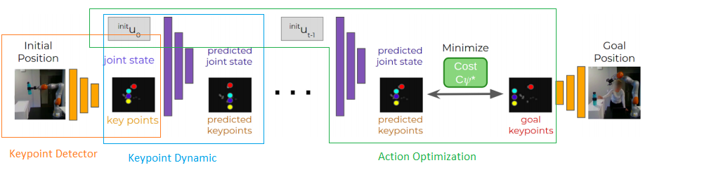
The optimization of action happened via Gradient-Based Visual Model Predictive Control Framework. It contains many components like keypoint detector, key points dynamics, etc. 

Keypoint Detector : detects the pixel position roughly corresponding to the object in the initial image.(low dimensional representation from an input RGB image)

Keypoint Dynamic : It predicts the key points and joint state at the next time step.

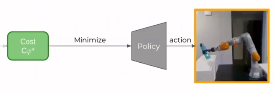
Action Optimization : gives the optimal set of actions that moves the object to its goal position by minimizing the cost function with respect to the actions using gradient descent.

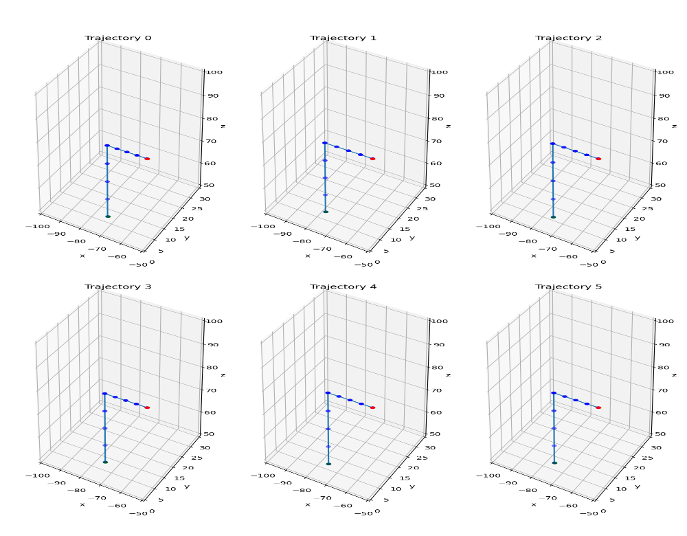
Results generated by the Proposed MBIRL Algorithm

Inferences drawn by learning from visual demonstration on different cost function parameterization like default cost, weighted cost, time-dependent cost and RBF weighted cost. Here default cost is just the difference between the predicted trajectory and the target.

Requirements & Installation

1. Python=3.7
2. Clone the Github repository via git.

 !git clone https://github.com/facebookresearch/LearningToLearn.git
 %cd LearningToLearn/ 

3. Install all the dependencies of MBIRL via :

!python setup.py develop

Simulation with ground truth keypoint predictions Demo

1. Generate the expert demonstrations by running the code line below:

!python mbirl/generate_expert_demo.py

You can check the data and visualization in LearningToLearn/mbirl/experiments/traj_data/

2. Run the model file by :

!python mbirl/experiments/run_model_based_irl.py

And check all the trajectories predicted during training in 

LearningToLearn/mbirl/experiments/model_data/placing/

3. Plot the loss functions. You have to uncomment the type of loss you want and train it again using the step 2. Line number 189 in mbirl/experiments/run_model_based_irl.py

1. Import all the required files and packages :

 import os, sys
 import torch
 import numpy as np
 import matplotlib.pyplot as plt
 from os.path import dirname, abspath
 from mbirl.keypoint_mpc import GroundTruthKeypointMPCWrapper
 from mbirl.learnable_costs import *
 import mbirl
 import warnings
 warnings.filterwarnings('ignore')
 EXP_FOLDER = os.path.join(mbirl.__path__[0], "experiments")
 traj_data_dir = os.path.join(EXP_FOLDER, 'traj_data')
 model_data_dir = os.path.join(EXP_FOLDER, 'model_data') 

2. Load the data saved during the training and testing(of all three loss functions for comparison).

 # Get data saved during training
 if not os.path.exists(
         f"{model_data_dir}/{experiment_type}_TimeDep") or not os.path.exists(
     f"{model_data_dir}/{experiment_type}_Weighted") or not os.path.exists(f"{model_data_dir}/{experiment_type}_RBF"):
     assert False, "Path does not exist"
 timedep = torch.load(f"{model_data_dir}/{experiment_type}_TimeDep")
 weighted = torch.load(f"{model_data_dir}/{experiment_type}_Weighted")
 rbf = torch.load(f"{model_data_dir}/{experiment_type}_RBF") 

3. Plot the loss function against the number of iterations of train data.

 # IRL Loss on train trajectories, as a function of cost function updates
 plt.figure()
 plt.plot(weighted['irl_loss_train'].detach(), color='orange', label="Weighted Ours")
 plt.plot(timedep['irl_loss_train'].detach(), color='green', label="Time Dep Weighted Ours")
 plt.plot(rbf['irl_loss_train'].detach(), color='violet', label="RBF Weighted Ours")
 plt.xlabel("iterations")
 plt.ylabel("IRL Loss on train")
 plt.ylim([0, 2000])
 plt.legend()
 plt.savefig(f"{model_data_dir}/{experiment_type}_IRL_loss_train.png") 

The output will be :

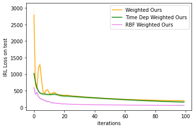
4. Plot the loss function against iterations on test data: The code snippet is available here.

EndNotes

This article briefed a model-based approach of inverse reinforcement learning to learn from a visual demonstration. The following method learns the cost function from the visual demonstration. This predicted cost function is used to regenerate the corresponding demonstration by using gradient-based visual model predictive control.

• Colab Notebook MBIRL Demo

Note : All the images/figures except for code output, are taken from official sources.

Official codes, documentation and tutorials are available at:

• Github
• Research Paper
• CoRL Conference