Series: Ensemble Methods

A Guide to AdaBoost: Boosting To Save The Day

AdaBoost is a very popular boosting technique. Here we'll cover the AdaBoost algorithm, its pros and cons, and implement it in Python using scikit-learn.

4 years ago • 11 min read

By Vihar Kurama

Today, machine learning is the premise of big innovations and promises to continue enabling companies to make the best decisions through accurate predictions. But what happens when the error susceptibility of these algorithms is high and unaccountable?

That is when Ensemble Learning saves the day!

AdaBoost is an ensemble learning method (also known as “meta-learning”) which was initially created to increase the efficiency of binary classifiers. AdaBoost uses an iterative approach to learn from the mistakes of weak classifiers, and turn them into strong ones.

In this article we'll learn about the following modules:

What is Ensemble Learning?
- Types of Ensemble Methods
- Boosting in Ensemble Methods
- Types of Boosting Algorithms
Unraveling AdaBoost
Pseudocode of AdaBoost
Implementation of AdaBoost Using Python
Advantages and Disadvantages of AdaBoost
Summary and Conclusion

You can run the code for this tutorial for free on the ML Showcase.

Launch Project For Free

Run on gradient

What Is Ensemble Learning?

Ensemble learning combines several base algorithms to form one optimized predictive algorithm. For example, a typical Decision Tree for classification takes several factors, turns them into rule questions, and given each factor, either makes a decision or considers another factor. The result of the decision tree can become ambiguous if there are multiple decision rules, e.g. if threshold to make a decision is unclear or we input new sub-factors for consideration. This is where Ensemble Methods comes at one's disposable. Instead of being hopeful on one Decision Tree to make the right call, Ensemble Methods take several different trees and aggregate them into one final, strong predictor.

Types Of Ensemble Methods

Ensemble Methods can be used for various reasons, mainly to:

Decrease Variance (Bagging)
Decrease Bias (Boosting)
Improve Predictions (Stacking)

Ensemble Methods can also be divided into two groups:

Sequential Learners, where different models are generated sequentially and the mistakes of previous models are learned by their successors. This aims at exploiting the dependency between models by giving the mislabeled examples higher weights (e.g. AdaBoost).
Parallel Learners, where base models are generated in parallel. This exploits the independence between models by averaging out the mistakes (e.g. Random Forest).

Boosting in Ensemble Methods

Just as humans learn from their mistakes and try not to repeat them further in life, the Boosting algorithm tries to build a strong learner (predictive model) from the mistakes of several weaker models. You start by creating a model from the training data. Then, you create a second model from the previous one by trying to reduce the errors from the previous model. Models are added sequentially, each correcting its predecessor, until the training data is predicted perfectly or the maximum number of models have been added.

Boosting basically tries to reduce the bias error which arises when models are not able to identify relevant trends in the data. This happens by evaluating the difference between the predicted value and the actual value.

Types of Boosting Algorithms

AdaBoost (Adaptive Boosting)
Gradient Tree Boosting
XGBoost

In this article, we will be focusing on the details of AdaBoost, which is perhaps the most popular boosting method.

Unraveling AdaBoost

AdaBoost (Adaptive Boosting) is a very popular boosting technique that aims at combining multiple weak classifiers to build one strong classifier. The original AdaBoost paper was authored by Yoav Freund and Robert Schapire.

A single classifier may not be able to accurately predict the class of an object, but when we group multiple weak classifiers with each one progressively learning from the others' wrongly classified objects, we can build one such strong model. The classifier mentioned here could be any of your basic classifiers, from Decision Trees (often the default) to Logistic Regression, etc.

Now we may ask, what is a "weak" classifier? A weak classifier is one that performs better than random guessing, but still performs poorly at designating classes to objects. For example, a weak classifier may predict that everyone above the age of 40 could not run a marathon but people falling below that age could. Now, you might get above 60% accuracy, but you would still be misclassifying a lot of data points!

Rather than being a model in itself, AdaBoost can be applied on top of any classifier to learn from its shortcomings and propose a more accurate model. It is usually called the “best out-of-the-box classifier” for this reason.

Let's try to understand how AdaBoost works with Decision Stumps. Decision Stumps are like trees in a Random Forest, but not "fully grown." They have one node and two leaves. AdaBoost uses a forest of such stumps rather than trees.

Stumps alone are not a good way to make decisions. A full-grown tree combines the decisions from all variables to predict the target value. A stump, on the other hand, can only use one variable to make a decision. Let's try and understand the behind-the-scenes of the AdaBoost algorithm step-by-step by looking at several variables to determine whether a person is "fit" (in good health) or not.

An Example of How AdaBoost Works

Step 1: A weak classifier (e.g. a decision stump) is made on top of the training data based on the weighted samples. Here, the weights of each sample indicate how important it is to be correctly classified. Initially, for the first stump, we give all the samples equal weights.

Step 2: We create a decision stump for each variable and see how well each stump classifies samples to their target classes. For example, in the diagram below we check for Age, Eating Junk Food, and Exercise. We'd look at how many samples are correctly or incorrectly classified as Fit or Unfit for each individual stump.

Step 3: More weight is assigned to the incorrectly classified samples so that they're classified correctly in the next decision stump. Weight is also assigned to each classifier based on the accuracy of the classifier, which means high accuracy = high weight!

Step 4: Reiterate from Step 2 until all the data points have been correctly classified, or the maximum iteration level has been reached.

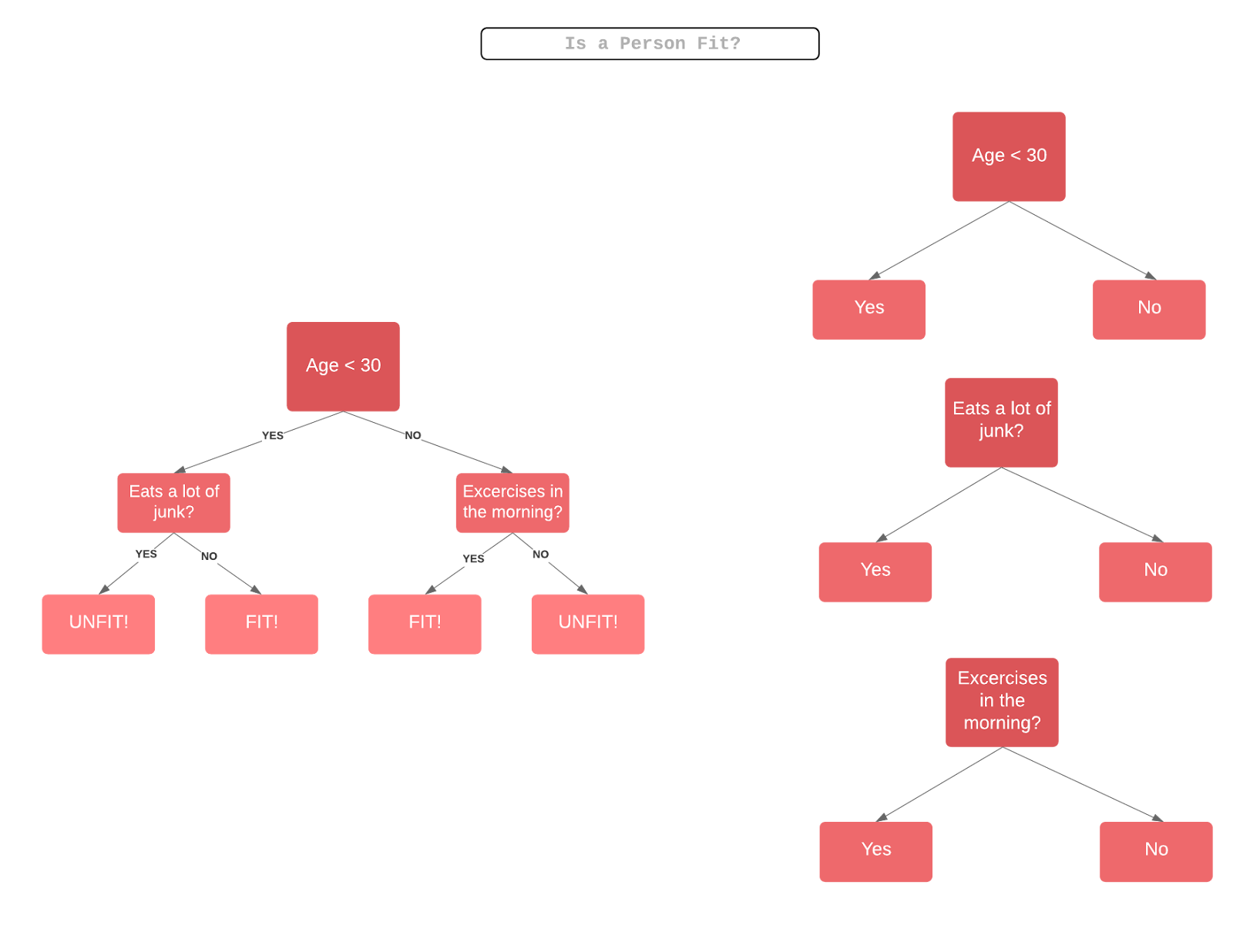
*Fully grown decision tree (left) vs three decision stumps (right)*

Note: Some stumps get more say in the classification than other stumps.

The Mathematics Behind AdaBoost

Here comes the hair-tugging part. Let's break AdaBoost down, step-by-step and equation-by-equation so that it's easier to comprehend.

Let's start by considering a dataset with N points, or rows, in our dataset.

In this case,

n is the dimension of real numbers, or the number of attributes in our dataset
x is the set of data points
y is the target variable which is either -1 or 1 as it is a binary classification problem, denoting the first or the second class (e.g. Fit vs Not Fit)

We calculate the weighted samples for each data point. AdaBoost assigns weight to each training example to determine its significance in the training dataset. When the assigned weights are high, that set of training data points are likely to have a larger say in the training set. Similarly, when the assigned weights are low, they have a minimal influence in the training dataset.

Initially, all the data points will have the same weighted sample w:

where N is the total number of data points.

The weighted samples always sum to 1, so the value of each individual weight will always lie between 0 and 1. After this, we calculate the actual influence for this classifier in classifying the data points using the formula:

Alpha is how much influence this stump will have in the final classification. Total Error is nothing but the total number of misclassifications for that training set divided by the training set size. We can plot a graph for Alpha by plugging in various values of Total Error ranging from 0 to 1.

Alpha vs Error Rate (Source: Chris McCormick)

Notice that when a Decision Stump does well, or has no misclassifications (a perfect stump!) this results in an error rate of 0 and a relatively large, positive alpha value.

If the stump just classifies half correctly and half incorrectly (an error rate of 0.5, no better than random guessing!) then the alpha value will be 0. Finally, when the stump ceaselessly gives misclassified results (just do the opposite of what the stump says!) then the alpha would be a large negative value.

After plugging in the actual values of Total Error for each stump, it's time for us to update the sample weights which we had initially taken as 1/N for every data point. We'll do this using the following formula:

In other words, the new sample weight will be equal to the old sample weight multiplied by Euler's number, raised to plus or minus alpha (which we just calculated in the previous step).

The two cases for alpha (positive or negative) indicate:

Alpha is positive when the predicted and the actual output agree (the sample was classified correctly). In this case we decrease the sample weight from what it was before, since we're already performing well.
Alpha is negative when the predicted output does not agree with the actual class (i.e. the sample is misclassified). In this case we need to increase the sample weight so that the same misclassification does not repeat in the next stump. This is how the stumps are dependent on their predecessors.

Pseudocode of AdaBoost

Initially set uniform example weights.

for Each base learner do:
Train base learner with a weighted sample.
Test base learner on all data.
Set learner weight with a weighted error.
Set example weights based on ensemble predictions.
end for

Implementation of AdaBoost Using Python

Step 1: Importing the Modules

As always, the first step in building our model is to import the necessary packages and modules.

In Python we have the AdaBoostClassifier and AdaBoostRegressor classes from the scikit-learn library. For our case we would import AdaBoostClassifier (since our example is a classification task). The train_test_split method is used to split our dataset into training and test sets. We also import datasets, from which we will use the the Iris Dataset.

from sklearn.ensemble import AdaBoostClassifier
from sklearn import datasets
from sklearn.model_selection import train_test_split
from sklearn import metrics

Step 2: Exploring the data

You can use any classification dataset, but here we'll use traditional Iris dataset for a multi-class classification problem. This dataset contains four features about different types of Iris flowers (sepal length, sepal width, petal length, petal width). The target is to predict the type of flower from three possibilities: Setosa, Versicolour, and Virginica. The dataset is available in the scikit-learn library, or you can also download it from the UCI Machine Learning Library.

Next, we make our data ready by loading it from the datasets package using the load_iris() method. We assign the data to the iris variable.

Further, we split our dataset into input variable X, which contains the features sepal length, sepal width, petal length, and petal width.

Y is our target variable, or the class that we have to predict: either Iris Setosa, Iris Versicolour, or Iris Virginica. Below is an example of what our data looks like.

iris = datasets.load_iris()
X = iris.data
y = iris.target
print(X)
print(Y)

Output:

[[5.1 3.5 1.4 0.2]
 [4.9 3.  1.4 0.2]
 [4.7 3.2 1.3 0.2]
 [4.6 3.1 1.5 0.2]
 [5.8 4.  1.2 0.2]
 [5.7 4.4 1.5 0.4]
. . . . 
. . . .
]
[0 0 0 0 0 0 0 0 0 0 0 0 0 0 0 0 0 0 0 0 0 0 0 0 0 0 0 0 0 0 0 0 0 0 0 0 
0 0 0 0 0 0 0 0 0 0 0 0 0 0 1 1 1 1 1 1 1 1 1 1 1 1 1 1 1 1 1 1 1 1 1 1 
1 1 1 1 1 1 1 1 1 1 1 1 1 1 1 1 1 1 1 1 1 1 1 1 1 1 1 1 2 2 2 2 2 2 2 2 
2 2 2 2 2 2 2 2 2 2 2 2 2 2 2 2 2 2 2 2 2 2 2 2 2 2 2 2 2 2 2 2 2 2 2 2 
2 2 2 2 2 2]

Step 3: Splitting the data

Splitting the dataset into training and testing datasets is a good idea to see if our model is classifying the data points correctly on unseen data.

X_train, X_test, y_train, y_test = train_test_split(X, y, test_size=0.3)

Here we split our dataset into 70% training and 30% test which is a common scenario.

Step 4: Fitting the Model

Building the AdaBoost Model. AdaBoost takes Decision Tree as its learner model by default. We make an AdaBoostClassifier object and name it abc. Few important parameters of AdaBoost are :

base_estimator: It is a weak learner used to train the model.
n_estimators: Number of weak learners to train in each iteration.
learning_rate: It contributes to the weights of weak learners. It uses 1 as a default value.

abc = AdaBoostClassifier(n_estimators=50,
                         learning_rate=1)

We then go ahead and fit our object abc to our training dataset. We call it a model.

model = abc.fit(X_train, y_train)

Step 5: Making the Predictions

Our next step would be to see how good or bad our model is to predict our target values.

y_pred = model.predict(X_test)

In this step, we take a sample observation and make a prediction on unseen data. Further, we use the predict() method on the model to check for the class it belongs to.

Step 6: Evaluating the model

The Model accuracy will tell us how many times our model predicts the correct classes.

print("Accuracy:", metrics.accuracy_score(y_test, y_pred))

Output:
Accuracy:0.8666666666666667

You get an accuracy of 86.66% – not bad. You can experiment with various other base learners like Support Vector Machine, Logistic Regression which might give you higher accuracy.

Advantages and Disadvantages of AdaBoost

AdaBoost has a lot of advantages, mainly it is easier to use with less need for tweaking parameters unlike algorithms like SVM. As a bonus, you can also use AdaBoost with SVM. Theoretically, AdaBoost is not prone to overfitting though there is no concrete proof for this. It could be because of the reason that parameters are not jointly optimized — stage-wise estimation slows down the learning process. To understand the math behind it in depth, you can follow this link.

AdaBoost can be used to improve the accuracy of your weak classifiers hence making it flexible. It has now being extended beyond binary classification and has found use cases in text and image classification as well.

A few Disadvantages of AdaBoost are :

Boosting technique learns progressively, it is important to ensure that you have quality data. AdaBoost is also extremely sensitive to Noisy data and outliers so if you do plan to use AdaBoost then it is highly recommended to eliminate them.

AdaBoost has also been proven to be slower than XGBoost.

Summary and Conclusion

In this article, we have discussed the various ways to understand the AdaBoost Algorithm. We started by introducing you to Ensemble Learning and it's various types to make sure that you understand where AdaBoost falls exactly. We discussed the pros and cons of the algorithm and gave you a quick demo on its implementation using Python.

AdaBoost is like a boon to improve the accuracy of our classification algorithms if used accurately. It is the first successful algorithm to boost binary classification. AdaBoost is increasingly being used in the industry and has found its place in Facial Recognition systems to detect if there is a face on the screen or not.

Hope this article was able to tingle your curiosity for you to research more in-depth about AdaBoost and various other Boosting algorithms.